Session 3

Review

Packages

How do you install a package from the R prompt, like readxl?

Answer

install.packages("readxl")

How do you load a package from the R prompt, like dplyr

Answer

library(dplyr)

How can you use RStudio to load a package?

Answer

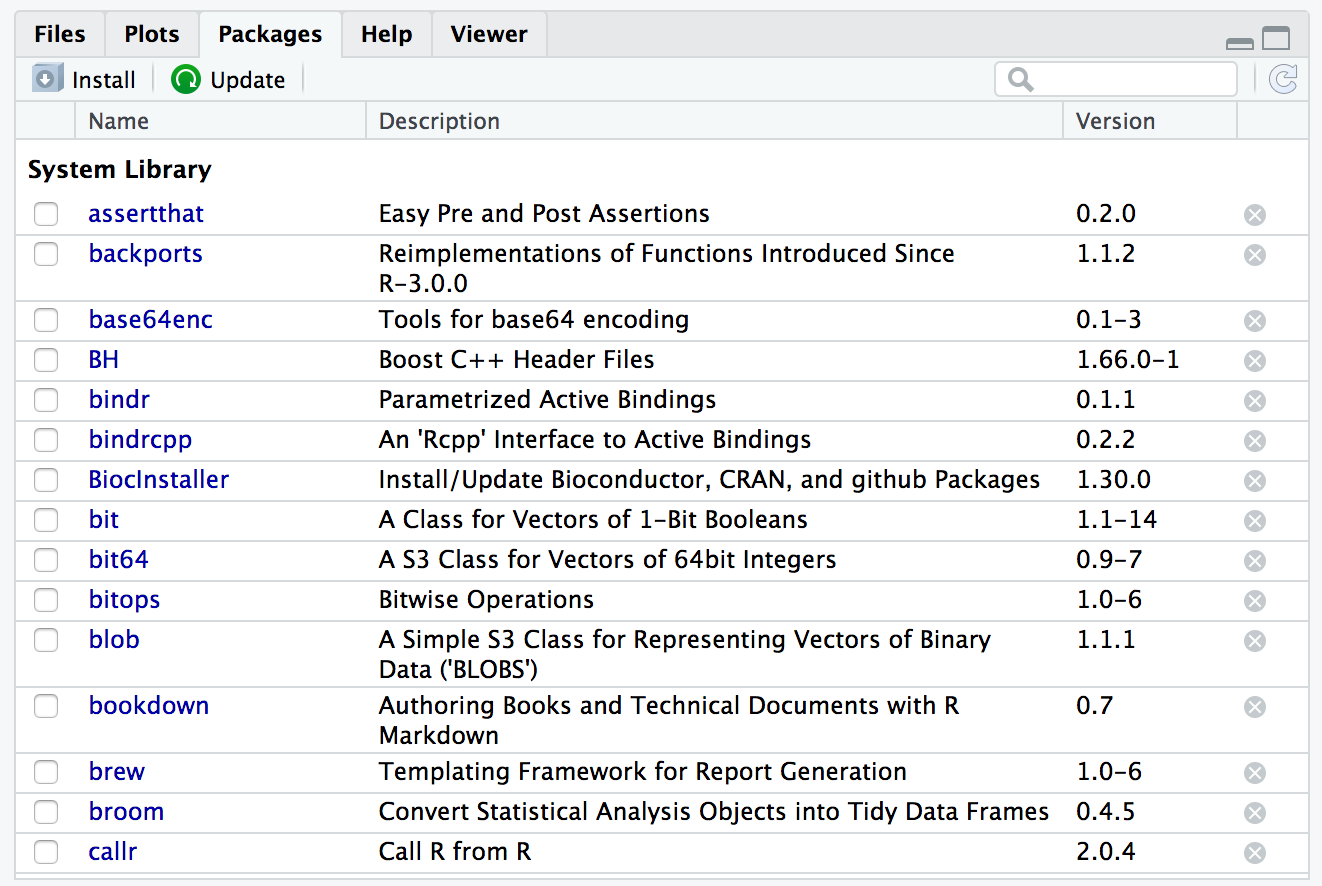
RStudio Packages Pane

Okay, but what is a package?

Answer

A package contains:

Functions
Documentation
Vignettes
Data

Data Types

What data type are each of the following?

Type	Example
	`1L`
	`3.14`, `1.23e-4`
	`"apple"`
	`TRUE`, `FALSE`
	`c(...)`
	`list(...)`
	`data.frame(...)`
	`data_frame(...)`
	`NA`
	`NULL`
	`factor(letters)`

Answer

integer, double, character, logical, vector, list, data.frame, tibble, N/A (missing), Null and factor

Run the following command. It will create 3 variables: x, y, and z. Without printing the variables, how can you tell what data type they are?

source("https://git.io/fNrm9")

Answer

Here’s the code that was run:

x <- 1:10
y <- setNames(sample(letters, 10), LETTERS[1:10])
z <- runif(10)
z[sample(1:10, 2)] <- NA

y

  A   B   C   D   E   F   G   H   I   J 
"x" "z" "g" "t" "o" "k" "v" "c" "l" "r"

 [1] 0.4577418        NA 0.9346722 0.2554288 0.4622928 0.9400145 0.9782264
 [8] 0.1174874 0.4749971        NA

class(x)

[1] "integer"

class(y)

[1] "character"

class(z)

[1] "numeric"

is.integer(x)

[1] TRUE

is.character(y)

[1] TRUE

is.na(z)

 [1] FALSE  TRUE FALSE FALSE FALSE FALSE FALSE FALSE FALSE  TRUE

Workspaces & RStudio Projects

In the last session, we created an RStudio project and an example R script.

Re-open the project we created (or create a new project).
What is the current working directory?
Use the File pane to navigate to your desktop (or another folder on your computer).
How can you quickly navigate back to the working directory?

Open example_single_patient.R from our previous session and add the following lines.

example <- data_frame(
  patient_id = patient_id,
  age_dx = age_at_diagnosis,
  age_visit = age_at_visit,
  tumor_size = tumor_size,
  site_code = site_code
)

Clear your workspace (quick refresher here) and then source the script.

View the tibble that is stored in example.

# A tibble: 5 x 5
  patient_id age_dx age_visit tumor_size site_code
       <dbl>  <dbl>     <int>      <dbl> <chr>    
1    5554321     54        54        9.5 C220     
2    5554321     54        55        9.5 C400     
3    5554321     54        56        9.7 C412     
4    5554321     54        57        9.9 C220     
5    5554321     54        58       10.1 C400

Functions

Functions that work with vectors

So far we’ve primarily seen vectors that operate on single values or that take single-valued arguments.

But as we’ve seen, R is a vectorized language.

Try using the following functions on the variables we created in example_single_patient.R in Session 2.

age_at_visit <- 54:58
tumor_size <- c(9.5, 9.5, 9.7, 9.9, 10.1)
site_code <- c("C220", "C400", "C412", "C220", "C400")

min(tumor_size)

[1] 9.5

max(tumor_size)

[1] 10.1

mean(tumor_size)

[1] 9.74

median(tumor_size)

[1] 9.7

var(tumor_size)

[1] 0.068

sd(tumor_size)

[1] 0.2607681

IQR(tumor_size)

[1] 0.4

Those functions all come from base R (standard R library).

The following functions are given to us from dplyr. We have dplyr loaded if we’ve run library(tidyverse), but I’ll include the dplyr:: first as a reminder that that’s where these functions come from.

dplyr::first(site_code)

[1] "C220"

dplyr::last(age_at_visit)

[1] 58

dplyr::nth(site_code, 2)

[1] "C400"

dplyr::n_distinct(site_code)

[1] 3

All of these functions return a single value. Try the following. What happens and why?

tumor_size * 10

[1]  95  95  97  99 101

age_at_visit - age_at_diagnosis

[1] 0 1 2 3 4

paste("Site Code:", site_code)

[1] "Site Code: C220" "Site Code: C400" "Site Code: C412" "Site Code: C220"
[5] "Site Code: C400"

Because R is vectorized, operations are applied to the whole vector.

Dot, dot, dot

R has a somewhat unique addition for writing and using functions: the dot-dot-dot (...).

The ... is used in two ways:

To allow you to include an unknown number of values.

paste <- function (..., sep = " ", collapse = NULL)

paste("a", "b", "c")

[1] "a b c"

paste("a", "b", "c", "d")

[1] "a b c d"

To allow you to pass arguments to an underlying function.

rep <- function (x, ...)  .Primitive("rep")

rep(1L, 4)

[1] 1 1 1 1

rep(1L, times = 4)

[1] 1 1 1 1

rep.int(1L, times = 4)

[1] 1 1 1 1

Before We Begin

Whenever you’re learning a new tool, for a long time you’re going to suck. It’s going to be very frustrating. But the good news is that that is typical, it’s something that happens to everyone, and it’s only temporary.

Unfortunately, there is no way to go from knowing nothing about a subject to knowing something about the subject … without going through a period of great frustration and much suckiness.

But remember, when you’re getting frustrated, that’s a good thing, it’s typical, it’s temporary. Keep pushing through and in time it will become second nature.

Hadley Wickham, UseR!2014

dplyr Basics

dplyr provides a wide range of functions for data manipulation and transformation. In this session, we’re going to cover 5 key dplyr functions:

Function	Action
`filter()`	Pick out observations by their values
`arrange()`	Reorder the rows
`select()`	Pick out variables by their names
`mutate()`	Create new variables using existing variables
`summarize()`	Collapse many values into a single summary

All dplyr verbs work similarly:

The first argument is a data frame.
Subsequent arguments describe how the verb will transform the data frame, using column names without "column_name"
The output is a new data frame.

`filter()`

filter(example, site_code == "C400")

# A tibble: 2 x 5
  patient_id age_dx age_visit tumor_size site_code
       <dbl>  <dbl>     <int>      <dbl> <chr>    
1    5554321     54        55        9.5 C400     
2    5554321     54        58       10.1 C400

filter(example, tumor_size > 9.5)

# A tibble: 3 x 5
  patient_id age_dx age_visit tumor_size site_code
       <dbl>  <dbl>     <int>      <dbl> <chr>    
1    5554321     54        56        9.7 C412     
2    5554321     54        57        9.9 C220     
3    5554321     54        58       10.1 C400

filter(example, age_visit < max(age_dx))

# A tibble: 0 x 5
# ... with 5 variables: patient_id <dbl>, age_dx <dbl>, age_visit <int>,
#   tumor_size <dbl>, site_code <chr>

Multiple arguments to filter() are combined with &:

filter(example, site_code == "C400", tumor_size > 9.5)

# A tibble: 1 x 5
  patient_id age_dx age_visit tumor_size site_code
       <dbl>  <dbl>     <int>      <dbl> <chr>    
1    5554321     54        58       10.1 C400

filter(example, site_code == "C400" & tumor_size > 9.5)

# A tibble: 1 x 5
  patient_id age_dx age_visit tumor_size site_code
       <dbl>  <dbl>     <int>      <dbl> <chr>    
1    5554321     54        58       10.1 C400

To build more complex filter combinations, use

Operation	Symbol
and	`&`
or	`\|`
not	`!`

Filtering for an item in a group

filter(example, site_code == "C412" | "C220") # doesn't work

Error in filter_impl(.data, quo): Evaluation error: operations are possible only for numeric, logical or complex types.

filter(example, site_code == "C412" | site_code == "C220")

# A tibble: 3 x 5
  patient_id age_dx age_visit tumor_size site_code
       <dbl>  <dbl>     <int>      <dbl> <chr>    
1    5554321     54        54        9.5 C220     
2    5554321     54        56        9.7 C412     
3    5554321     54        57        9.9 C220

filter(example, site_code %in% c("C412", "C220"))

# A tibble: 3 x 5
  patient_id age_dx age_visit tumor_size site_code
       <dbl>  <dbl>     <int>      <dbl> <chr>    
1    5554321     54        54        9.5 C220     
2    5554321     54        56        9.7 C412     
3    5554321     54        57        9.9 C220

Missing values

Filtering can be tricky when there are missing values – NA. Or sometimes, you’re trying to find the missing values.

It’s important to keep in mind that NAs are “contagious” in R, meaning that the result of almost any operation involving an NA will be an NA.

NA > 42

[1] NA

1 == NA

[1] NA

NA + 2

[1] NA

NA / 3

[1] NA

NA == NA

[1] NA

Here’s an example that helps to illustrate why NA == NA isn’t TRUE.

# Let x be Mary's age. We don't know how old she is.
x <- NA

# Let y be John's age. We don't know how old he is.
y <- NA

# Are John and Mary the same age?
x == y

[1] NA

filter() keeps only the rows where the condition is TRUE and drops the rows where it is FALSE or NA.

df <- tibble(x = c(1, NA, 3))
filter(df, x > 1)

# A tibble: 1 x 1
      x
  <dbl>
1     3

filter(df, is.na(x) | x > 1)

# A tibble: 2 x 1
      x
  <dbl>
1    NA
2     3

`arrange()`

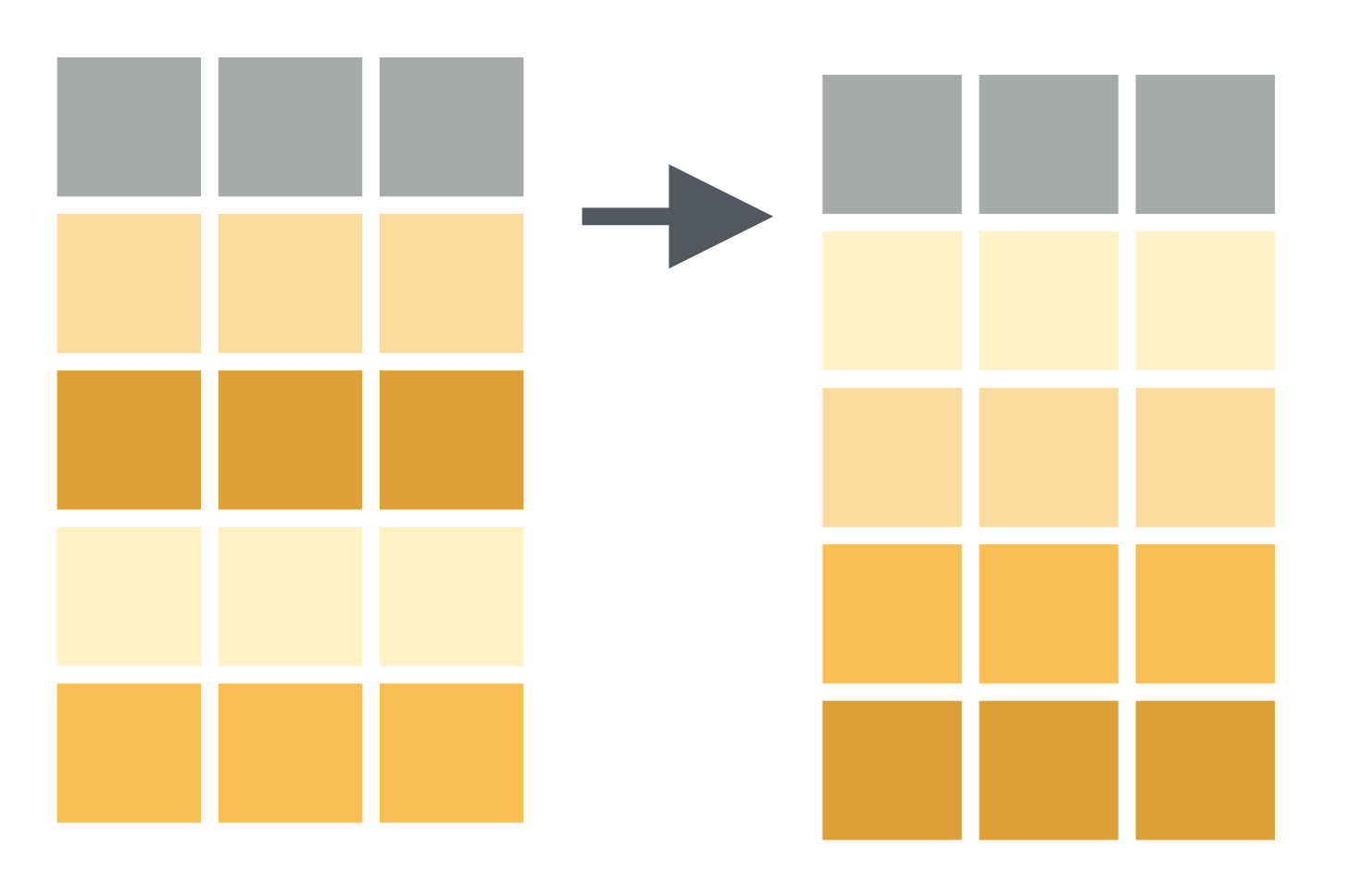
To arrange, or sort, the rows according to values in a given column, use arrange().

arrange(example, site_code)

# A tibble: 5 x 5
  patient_id age_dx age_visit tumor_size site_code
       <dbl>  <dbl>     <int>      <dbl> <chr>    
1    5554321     54        54        9.5 C220     
2    5554321     54        57        9.9 C220     
3    5554321     54        55        9.5 C400     
4    5554321     54        58       10.1 C400     
5    5554321     54        56        9.7 C412

arrange(example, desc(site_code))

# A tibble: 5 x 5
  patient_id age_dx age_visit tumor_size site_code
       <dbl>  <dbl>     <int>      <dbl> <chr>    
1    5554321     54        56        9.7 C412     
2    5554321     54        55        9.5 C400     
3    5554321     54        58       10.1 C400     
4    5554321     54        54        9.5 C220     
5    5554321     54        57        9.9 C220

arrange(example, site_code, tumor_size)

# A tibble: 5 x 5
  patient_id age_dx age_visit tumor_size site_code
       <dbl>  <dbl>     <int>      <dbl> <chr>    
1    5554321     54        54        9.5 C220     
2    5554321     54        57        9.9 C220     
3    5554321     54        55        9.5 C400     
4    5554321     54        58       10.1 C400     
5    5554321     54        56        9.7 C412

arrange(example, desc(tumor_size), site_code)

# A tibble: 5 x 5
  patient_id age_dx age_visit tumor_size site_code
       <dbl>  <dbl>     <int>      <dbl> <chr>    
1    5554321     54        58       10.1 C400     
2    5554321     54        57        9.9 C220     
3    5554321     54        56        9.7 C412     
4    5554321     54        54        9.5 C220     
5    5554321     54        55        9.5 C400

`select()`

select(example, age_dx, tumor_size)

# A tibble: 5 x 2
  age_dx tumor_size
   <dbl>      <dbl>
1     54        9.5
2     54        9.5
3     54        9.7
4     54        9.9
5     54       10.1

select(example, age_dx:tumor_size)

# A tibble: 5 x 3
  age_dx age_visit tumor_size
   <dbl>     <int>      <dbl>
1     54        54        9.5
2     54        55        9.5
3     54        56        9.7
4     54        57        9.9
5     54        58       10.1

select(example, -(patient_id:age_visit))

# A tibble: 5 x 2
  tumor_size site_code
       <dbl> <chr>    
1        9.5 C220     
2        9.5 C400     
3        9.7 C412     
4        9.9 C220     
5       10.1 C400

Helper functions for `select()`

select(example, starts_with("age"))

# A tibble: 5 x 2
  age_dx age_visit
   <dbl>     <int>
1     54        54
2     54        55
3     54        56
4     54        57
5     54        58

select(example, ends_with("id"))

# A tibble: 5 x 1
  patient_id
       <dbl>
1    5554321
2    5554321
3    5554321
4    5554321
5    5554321

select(example, contains("code"))

# A tibble: 5 x 1
  site_code
  <chr>    
1 C220     
2 C400     
3 C412     
4 C220     
5 C400

Renaming

select(example, code = site_code)

# A tibble: 5 x 1
  code 
  <chr>
1 C220 
2 C400 
3 C412 
4 C220 
5 C400

rename(example, code = site_code)

# A tibble: 5 x 5
  patient_id age_dx age_visit tumor_size code 
       <dbl>  <dbl>     <int>      <dbl> <chr>
1    5554321     54        54        9.5 C220 
2    5554321     54        55        9.5 C400 
3    5554321     54        56        9.7 C412 
4    5554321     54        57        9.9 C220 
5    5554321     54        58       10.1 C400

`mutate()`

mutate(example, follow_up = age_visit - age_dx)

# A tibble: 5 x 6
  patient_id age_dx age_visit tumor_size site_code follow_up
       <dbl>  <dbl>     <int>      <dbl> <chr>         <dbl>
1    5554321     54        54        9.5 C220              0
2    5554321     54        55        9.5 C400              1
3    5554321     54        56        9.7 C412              2
4    5554321     54        57        9.9 C220              3
5    5554321     54        58       10.1 C400              4

mutate(example, elapsed = age_visit - min(age_visit))

# A tibble: 5 x 6
  patient_id age_dx age_visit tumor_size site_code elapsed
       <dbl>  <dbl>     <int>      <dbl> <chr>       <dbl>
1    5554321     54        54        9.5 C220            0
2    5554321     54        55        9.5 C400            1
3    5554321     54        56        9.7 C412            2
4    5554321     54        57        9.9 C220            3
5    5554321     54        58       10.1 C400            4

mutate(example, 
       tumor_size = tumor_size * 10, 
       tumor_size_mm = tumor_size *100)

# A tibble: 5 x 6
  patient_id age_dx age_visit tumor_size site_code tumor_size_mm
       <dbl>  <dbl>     <int>      <dbl> <chr>             <dbl>
1    5554321     54        54         95 C220               9500
2    5554321     54        55         95 C400               9500
3    5554321     54        56         97 C412               9700
4    5554321     54        57         99 C220               9900
5    5554321     54        58        101 C400              10100

Recoding or conditionally changing values

Often you’ll want to replace certain values of a variable with another value. There are several helpful functions provided by dplyr that let you do this, including:

recode(): Replace character values with "old" = "new".

var = recode(var, "old" = "new", "OLD" = "new")

if_else(): Use logical statements to change the value.

var = if_else(CONDITION, VALUE_IF_TRUE, VALUE_IF_FALSE)

mutate(example, site_code = recode(site_code, "C412" = "C999"))

# A tibble: 5 x 5
  patient_id age_dx age_visit tumor_size site_code
       <dbl>  <dbl>     <int>      <dbl> <chr>    
1    5554321     54        54        9.5 C220     
2    5554321     54        55        9.5 C400     
3    5554321     54        56        9.7 C999     
4    5554321     54        57        9.9 C220     
5    5554321     54        58       10.1 C400

mutate(example, tumor_size = if_else(site_code == "C400", tumor_size * 100, tumor_size))

# A tibble: 5 x 5
  patient_id age_dx age_visit tumor_size site_code
       <dbl>  <dbl>     <int>      <dbl> <chr>    
1    5554321     54        54        9.5 C220     
2    5554321     54        55      950   C400     
3    5554321     54        56        9.7 C412     
4    5554321     54        57        9.9 C220     
5    5554321     54        58     1010   C400

`summarize()`

summarize(example, min(age_dx))

# A tibble: 1 x 1
  `min(age_dx)`
          <dbl>
1            54

summarize(example, max_tumor_size = max(tumor_size))

# A tibble: 1 x 1
  max_tumor_size
           <dbl>
1           10.1

summarize(example, tumor_size_median = median(tumor_size),tumor_size_mean = mean(tumor_size), age_visit = max(age_visit))

# A tibble: 1 x 3
  tumor_size_median tumor_size_mean age_visit
              <dbl>           <dbl>     <dbl>
1               9.7            9.74        58

`group_by()` & `summarize()`

example_grp <- group_by(example, site_code)
summarize(example_grp, 
  tumor_size_mean = mean(tumor_size), 
  age_mean = mean(age_dx))

# A tibble: 3 x 3
  site_code tumor_size_mean age_mean
  <chr>               <dbl>    <dbl>
1 C220                  9.7       54
2 C400                  9.8       54
3 C412                  9.7       54

example_grp <- group_by(example, site_code, patient_id)
summarize(example_grp, 
  tumor_size_mean = mean(tumor_size), 
  age_mean = mean(age_dx))

# A tibble: 3 x 4
# Groups:   site_code [?]
  site_code patient_id tumor_size_mean age_mean
  <chr>          <dbl>           <dbl>    <dbl>
1 C220         5554321             9.7       54
2 C400         5554321             9.8       54
3 C412         5554321             9.7       54

`group_by()` & `count()`

count(example, site_code)

# A tibble: 3 x 2
  site_code     n
  <chr>     <int>
1 C220          2
2 C400          2
3 C412          1

count(example, patient_id)

# A tibble: 1 x 2
  patient_id     n
       <dbl> <int>
1    5554321     5

# Groups: site_code, patient_id
count(example_grp)

# A tibble: 3 x 3
# Groups:   site_code, patient_id [3]
  site_code patient_id     n
  <chr>          <dbl> <int>
1 C220         5554321     2
2 C400         5554321     2
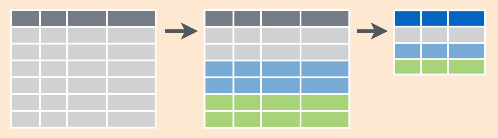
3 C412         5554321     1

Combining dplyr Verbs

Let’s say we want to calculate the average age and tumor size (in cm) by site code for each patient.

To do this we’ll take our example data and

Group by site_code and patient_id
Convert tumor size from cm to mm
Summarize tumor_size and age_dx by their average.

In dplyr speak:

ex1 <- group_by(example, site_code, patient_id)
ex2 <- mutate(ex1, tumor_size = tumor_size * 10)
ex3 <- summarize(ex2, 
  tumor_size_mean = mean(tumor_size), 
  age_mean = mean(age_dx))
ex3

# A tibble: 3 x 4
# Groups:   site_code [?]
  site_code patient_id tumor_size_mean age_mean
  <chr>          <dbl>           <dbl>    <dbl>
1 C220         5554321              97       54
2 C400         5554321              98       54
3 C412         5554321              97       54

Notice that the output from each step is the input to the next step. Also, we don’t really need ex1 or ex2, we just want the output which we’ve saved as ex3.

To make this much cleaner we can use the pipe operator.

example %>% 
  group_by(site_code, patient_id) %>% 
  mutate(tumor_size = tumor_size * 10) %>% 
  summarize(
    tumor_size_mean = mean(tumor_size),
    age_mean = mean(age_dx)
  )

# A tibble: 3 x 4
# Groups:   site_code [?]
  site_code patient_id tumor_size_mean age_mean
  <chr>          <dbl>           <dbl>    <dbl>
1 C220         5554321              97       54
2 C400         5554321              98       54
3 C412         5554321              97       54

The pipe operator looks like this

%>%

You can type it with

Ctrl + Shift + M (Windows)

Cmd + Shift + M (Mac)

You say it like

…and then…

Re-read the code above:

Take example and then…
Group by and then…
Mutate and then…
Summarize

The pipe operator is now ubiquitous in modern R code, but it’s not part of the R language.

Make sure that you load tidyverse or dplyr first!

Your turn!

Use the pipe operator and dplyr verbs to complete the following task:

Use the example dataset
Filter out tumors smaller than 9.7
Calculate follow_up time as the number of years between diagnosis and the patient’s visit
Rename the site_code column to code.

Session 3

August 1, 2018

Links

Review

Packages

Data Types

Workspaces & RStudio Projects

Overview

Functions

Functions that work with vectors

Dot, dot, dot

Before We Begin

Before We Begin

dplyr Basics

`filter()`

Filtering for an item in a group

Missing values

`arrange()`

`select()`

Helper functions for `select()`

Renaming

`mutate()`

Recoding or conditionally changing values

`summarize()`

`group_by()` & `summarize()`

`group_by()` & `count()`

Combining dplyr Verbs

Your turn!

Session 3

August 1, 2018

Links

Review

Packages

Data Types

Workspaces & RStudio Projects

Overview

Functions

Functions that work with vectors

Dot, dot, dot

Before We Begin

Before We Begin

dplyr Basics

filter()

Filtering for an item in a group

Missing values

arrange()

select()

Helper functions for select()

Renaming

mutate()

Recoding or conditionally changing values

summarize()

group_by() & summarize()

group_by() & count()

Combining dplyr Verbs

Your turn!

`filter()`

`arrange()`

`select()`

Helper functions for `select()`

`mutate()`

`summarize()`

`group_by()` & `summarize()`

`group_by()` & `count()`