Session 6
August 22, 2018
Homework Review
Review the homework from Session 5.
You can check out the approach I took in this page. There is more than one way to accomplish each task, so it’s okay if your code looks different!
- What parts of these tasks were difficult?
- Which parts did you find easy?
- What questions did you have as you worked?
- Were you able to find the answers to any of these questions?
Overview
- Tidying Data
- Group discussion: messy data sets
- Joins
- Review Joins
- Group work joining data
- Working with dates and times
Tidying Data
The three rules of tidy data
Columns represent separate variables
Rows represent individual observations
Observational units form tables
Why tidy data?
Each of the following tables contains the same five variables: mrn, sequence, age, tumor_size, tumor_unit.
How easy would it be to calculate average tumor size for each patient? What problems would you face if your data were formatted like the examples below?
Example 1
# A tibble: 20 x 4
      mrn sequence type       value
    <int>    <int> <chr>      <chr>
 1 289034        1 age        47
 2 289034        1 tumor_size 0.9 cm
 3 289034        2 age        47
 4 289034        2 tumor_size 999 mm
 5 290660        1 age        49
 6 290660        1 tumor_size 30 mm
 7 290660        2 age        49
 8 290660        2 tumor_size 999 mm
 9 341050        1 age        61
10 341050        1 tumor_size 999 mm
11 341050        2 age        70
12 341050        2 tumor_size 2.1 cm
13 385615        1 age        71
14 385615        1 tumor_size 12 mm
15 385615        2 age        71
16 385615        2 tumor_size 2 cm
17 550955        1 age        43
18 550955        1 tumor_size 2.5 cm
19 550955        2 age        43
20 550955        2 tumor_size 998 mm
Example 2
# A tibble: 10 x 4
      mrn age    tumor_size tumor_unit
    <int> <chr>       <dbl> <chr>
 1 289034 47 (1)        0.9 cm
 2 289034 47 (2)      999   mm
 3 290660 49 (1)       30   mm
 4 290660 49 (2)      999   mm
 5 341050 61 (1)      999   mm
 6 341050 70 (2)        2.1 cm
 7 385615 71 (1)       12   mm
 8 385615 71 (2)        2   cm
 9 550955 43 (1)        2.5 cm
10 550955 43 (2)      998   mm
Example 3
# A tibble: 5 x 3
     mrn   `1`   `2`
   <int> <int> <int>
1 289034    47    47
2 290660    49    49
3 341050    61    70
4 385615    71    71
5 550955 43 43# A tibble: 5 x 3
mrn `1` `2`
<int> <chr> <chr>
1 289034 0.9 cm 999 mm
2 290660 30 mm 999 mm
3 341050 999 mm 2.1 cm
4 385615 12 mm 2 cm
5 550955 2.5 cm 998 mmExample 4
# A tibble: 4 x 11
  var   `289034` `289034` `290660` `290660` `341050` `341050` `385615`
  <chr> <chr>    <chr>    <chr>    <chr>    <chr>    <chr>    <chr>
1 sequ… 1        2        1        2        1        2        1
2 age   47       47       49       49       61       70       71
3 tumo… 0.9      999.0    30.0     999.0    999.0    2.1      12.0
4 tumo… cm       mm       mm       mm       mm       cm       mm
# ... with 3 more variables: `385615` <chr>, `550955` <chr>,
#   `550955` <chr>
Tidying Data
Most data isn’t tidy: often data is organized for something other than analysis. For example, the data may be structured in a way that’s easiest for data entry or so that all of the data fits on a single page.
First, ask yourself (or the person who created the data):
What are the variables?
What are the observations?
Sometimes, a variable is spread across multiple columns. Othertimes, an observation is scattered across multiple rows.
The tidyr packages is part of the tidyverse and loaded with library(tidyverse).
gather()
Use gather() to gather the values of a variable that are spread across columns.
The key is the name of the variable that will hold the values that are currently used as column names. The value is the name of the variables that holds the values in those columns.
# A tibble: 5 x 3
     mrn   `1`   `2`
   <int> <int> <int>
1 289034    47    47
2 290660    49    49
3 341050    61    70
4 385615    71    71
5 550955 43 43# A tibble: 10 x 3
mrn sequence age
<int> <chr> <int>
1 289034 1 47
2 290660 1 49
3 341050 1 61
4 385615 1 71
5 550955 1 43
6 289034 2 47
7 290660 2 49
8 341050 2 70
9 385615 2 71
10 550955 2 43spread()
spread() is the inverse of gather(). The values of the variable given as key will be the new column names that will contain the values in value.
# A tibble: 20 x 4
      mrn sequence type       value
    <int>    <int> <chr>      <chr>
 1 289034        1 age        47
 2 289034        1 tumor_size 0.9 cm
 3 289034        2 age        47
 4 289034        2 tumor_size 999 mm
 5 290660        1 age        49
 6 290660        1 tumor_size 30 mm
 7 290660        2 age        49
 8 290660        2 tumor_size 999 mm
 9 341050        1 age        61
10 341050        1 tumor_size 999 mm
11 341050        2 age        70
12 341050        2 tumor_size 2.1 cm
13 385615        1 age        71
14 385615        1 tumor_size 12 mm
15 385615        2 age        71
16 385615        2 tumor_size 2 cm
17 550955        1 age        43
18 550955        1 tumor_size 2.5 cm
19 550955        2 age        43
20 550955 2 tumor_size 998 mm# A tibble: 10 x 4
mrn sequence age tumor_size
<int> <int> <chr> <chr>
1 289034 1 47 0.9 cm
2 289034 2 47 999 mm
3 290660 1 49 30 mm
4 290660 2 49 999 mm
5 341050 1 61 999 mm
6 341050 2 70 2.1 cm
7 385615 1 71 12 mm
8 385615 2 71 2 cm
9 550955 1 43 2.5 cm
10 550955 2 43 998 mm Animated
Quick Review
Which function would you use to transform this data into tidy format?
Working with Dates
To work with dates, we need another packges from the tidyverse called lubridate. This package isn’t loaded by default, so you’ll need to run
Attaching package: 'lubridate'The following object is masked from 'package:base':
dateAbout dates, times and date-times
2006-01-02 03:04:05A date-time is a point in time, stored as the number of seconds since 1970-01-01 00:00:00 UTC. Note that a date-time also understands time zones.
[1] "2006-01-02 03:04:05 UTC"A date is a day and is stored as the number of days since 1970-01-01.
[1] "2006-01-02"An hms time is stored as the number of seconds since 00:00:00.
03:04:05Converting strings to date-times
lubridate has a number of functions that convert strings to date-times. The functions are named so that they match the order of the date components in the string. The the string doesn’t include time, a date is returned rather than a date-time.
| element | letter |
|---|---|
| year | y |
| month | m |
| day | d |
| hour | h |
| minute | m |
| second | s |
[1] "2006-01-02 03:04:05 UTC"[1] "2006-01-02 03:04:00 UTC"[1] "2006-01-02"[1] "2006-01-02 03:04:00 UTC"[1] "2006-01-02 03:04:00 UTC"[1] "2006-01-02"[1] "2006-01-02 03:04:00 UTC"[1] "2006-01-02"Getting and Setting Date Components
You can get or set a date component with the singular noun describing the date element.
[1] "2006-01-02"[1] 2006[1] 1[1] 2006[1] 1[1] 1[1] 2[1] 2[1] Mon
Levels: Sun < Mon < Tue < Wed < Thu < Fri < Sat[1] Monday
7 Levels: Sunday < Monday < Tuesday < Wednesday < Thursday < ... < Saturday[1] 3[1] 4[1] 5For all of the above you can also use this syntax to change the value.
[1] "2006-01-07 03:04:05 UTC"Moving the date-time
If you want to adjust a date-time on the timeline, you can add or subtract time periods, like 2 years. These functions are all named after the plural nouns.
[1] "2010-01-02 03:04:05 UTC"[1] "2006-05-02 03:04:05 UTC"[1] "2005-12-29 03:04:05 UTC"[1] "2006-01-02 02:04:05 UTC"[1] "2006-01-02 03:24:05 UTC"Durations and Comparing date-times
[1] FALSE[1] TRUETime difference of 397.0424 daysError in `+.POSIXt`(x, y): binary '+' is not defined for "POSIXt" objectsTime difference of 397.0424 days[1] 397Time difference of 397 days[1] 397Rounding Dates
x <- ymd_hms("2006-01-02 03:04:05")
y <- ymd_hms("2007-02-03 04:05:06")

# Round to nearest unit
round_date(x, unit = "minute")
[1] "2006-01-02 03:04:00 UTC"[1] "2007-02-01 UTC"[1] "2006-01-02 03:00:00 UTC"[1] "2006-01-02 UTC"[1] "2007-02-03 05:00:00 UTC"[1] "2007-02-04 UTC"[1] "2005-12-31 03:04:05 UTC"[1] "2006-01-01 03:04:05 UTC"[1] "2006-01-01 UTC"Time Zones
[1] "2006-01-01 22:04:05 EST"[1] "2006-01-02 03:04:05 EST" [1] "US/Alaska" "US/Aleutian" "US/Arizona"
[4] "US/Central" "US/East-Indiana" "US/Eastern"
[7] "US/Hawaii" "US/Indiana-Starke" "US/Michigan"
[10] "US/Mountain" "US/Pacific" "US/Pacific-New"
[13] "US/Samoa" Assignment
Review: Two-Table dplyr verbs
Keys
What are the two types of keys?
Answer
A primary key uniquely identifies an observation in its own table.
- A foreign key uniquely identifies an observation in another table.
Joins
I highly encourage you to read the chapter on Relational Data in the R4DS book.
You can also review all of the join animations by visiting my page on tidy animated verbs.
Joins Review
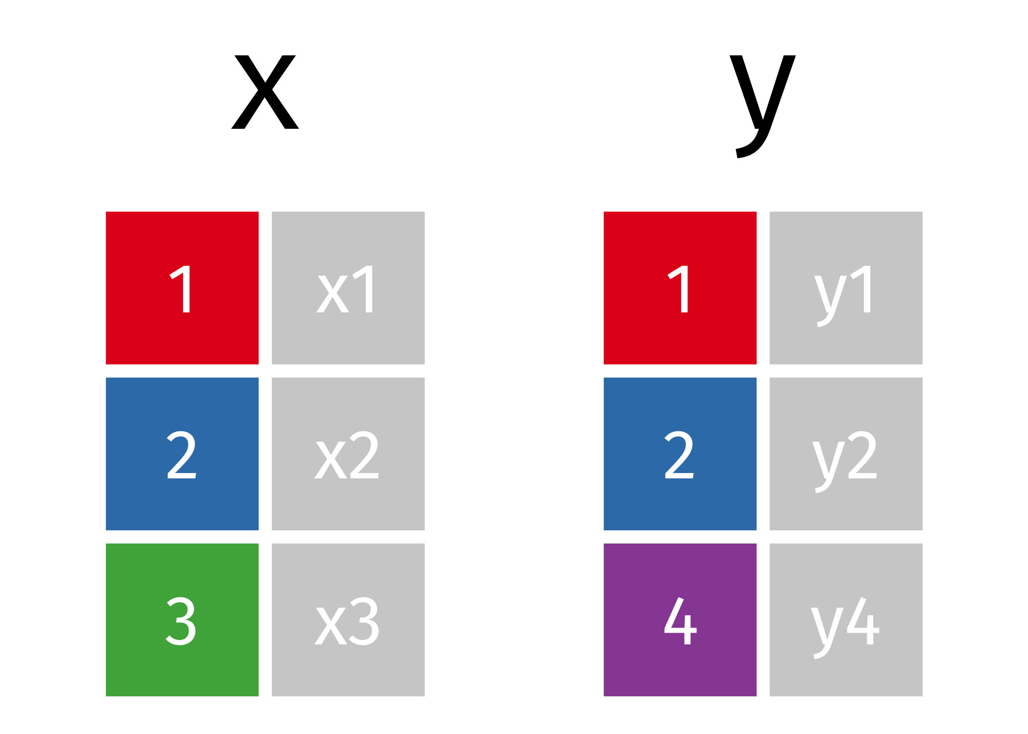
Mutating Joins
Filtering Joins
Homework
We’ll use the Breast Cancer Registry Data from Session 4. I’ve started writing the script with some tips and hints, which you can download from the Session 6 materials page. Or, if you’d like to start blind, you can use the code in Import Data below to get started.
Import Data
library(tidyverse)
# If you don't have the data in your working directory, you can download it by
# uncommenting and running the two lines below.
# download.file("https://git.io/fATNV", "CancerRegistryData.csv")
# download.file("https://git.io/fATNo", "CancerRegistryDataPatients.csv")

cr_patients <- read_csv(
  "CancerRegistryDataPatients.csv",
  col_types = cols(`Date Last Patient Contact/Dead` = col_date(format = "%m/%d/%y"))
)

cr <- read_csv(
  "CancerRegistryData.csv",
  col_types = cols(
    `Date Last Patient Contact/Dead` = col_date(format = "%m/%d/%y"),
    `Date of Diagnosis` = col_date(format = "%m/%d/%y")
  )
)
Task 1
Merge the two data sets to add the patient information to their diagnosis records.
Task 2
Find deceased patients at least 75 years or older. Create a data frame containing their patient information and all of their diagnosis records.
Task 3
Find the diagnosis records of the African American patients.
Bonus: Find the diagnosis records of married African American patients using two joins.
Task 4
First, verify that all patients in the diagnosis records data set cr appearin the patient information data set using anti_join
Then, find all patients who have had more than one cancer diagnosis and create a data frame with only their patient information, using semi_join().
Task 5
Find patients who were last contacted in 2017 and merge their patient information with their diagnosis records. Transform all dates to be the number of days since their earliest diagnosis.