Setup
The fcds package doesn’t include data from the FCDS Florida Cancer Registry. Please visit the FCDS Data Request page to request the most recent Florida Statewide Cancer Registry data.
Once you have downloaded the data, you can use fcds to pre-process and import the FCDS data into R.
fcds <- fcds_import("STAT_dataset_2018.dat")
The imported, pre-processed data is automatically cached in the .fcds directory in your home directory for later use. Calling fcds_load() will re-load the cached data.
fcds <- fcds_load()
You can customize the folder where the cached data files are stored; see ?fcds_default_data_path for more information.
You can also list the files currently stored in the data cache with fcds_cache_ls() and you can clean outdated files with fcds_cache_clean(), which by default retains the most recently imported FCDS data file.
Example Data
If you don’t have access to the FCDS data, we have provided a small example data set with similar properties to the FCDS data, but without any overlap in the attributes of cases.
fcds <- fcds::fcds_example

fcds[1:5, ]
#> # A tibble: 5 x 36
#>   patient_id year_group year  cancer_status cancer_site_gro… cancer_site_spe…
#>        <dbl> <fct>      <chr> <fct>         <fct>            <fct>
#> 1      10001 1982-1986  1984  Unknown       Colon excluding… "Cecum, Appendi…
#> 2      10002 1982-1986  1984  Evidence of … Breast           "Breast"
#> 3      10003 1982-1986  1984  Evidence of … Lung and Bronch… "Lung & Bronchu…
#> 4      10004 1982-1986  1984  No evidence … Colon excluding… "Cecum, Appendi…
#> 5      10005 1982-1986  1984  Unknown       Colon excluding… "Cecum, Appendi…
#> # … with 30 more variables: cancer_confirmation <fct>, age_group <fct>,
#> #   race <fct>, sex <fct>, origin <fct>, marital_status <fct>,
#> #   county_name <fct>, county_fips <chr>, state <fct>, florida_resident <lgl>,
#> #   country <fct>, birth_country <fct>, birth_state <fct>, primary_payer <fct>,
#> #   cancer_reporting_source <fct>, cancer_ICDO3_conversion <fct>,
#> #   cancer_laterality <fct>, cancer_grade <fct>, cancer_ICDO3_histology <chr>,
#> #   cancer_ICDO3_behavior <fct>, cancer_ICDO3_morphology <chr>,
#> #   seer_stage_1977 <fct>, seer_stage_2000 <fct>, seer_stage <fct>,
#> #   seer_stage_derived_1977 <fct>, seer_stage_derived_2000 <fct>,
#> #   tobacco_cigarette <fct>, tobacco_other <fct>, tobacco_smokeless <fct>,
#> #   tobacco_nos <fct>
Looking up FCDS Values
FCDS Constants
Lookup the values of variables in the imported data (referred to as a labels of the original data value) with fcds_const()
fcds_const(NULL)
#> Valid fcds_const() variables include: "year_group", "cancer_status", "cancer_site_group", "cancer_site_specific", "cancer_confirmation", "age_group", "race", "sex", "origin", "marital_status", "county_name", "state", "country", "birth_country", "birth_state", "primary_payer", "cancer_reporting_source", "cancer_ICDO3_conversion", "cancer_laterality", "cancer_grade", "cancer_ICDO3_behavior", "seer_stage_1977", "seer_stage_2000", "seer_stage_derived_1977", "seer_stage_derived_2000", "tobacco_cigarette", "tobacco_other", "tobacco_smokeless", "tobacco_nos", "moffitt_catchment"

fcds_const("cancer_status")
#> [1] "No evidence of tumor" "Evidence of tumor"    "Unknown"
If you supply full = TRUE, the original column name (name_original) and value from the FCDS data will be reported alongsize the cleaned column name (name_clean) and the value label used by the fcds package.
fcds_const("cancer_site_group", full = TRUE)
#> # A tibble: 41 x 4
#>    name_clean        name_original   value label
#>    <chr>             <chr>           <chr> <chr>
#>  1 cancer_site_group FCDS_Site_Group 0110  Oral Cavity and Pharynx
#>  2 cancer_site_group FCDS_Site_Group 0011  Esophagus
#>  3 cancer_site_group FCDS_Site_Group 0012  Stomach
#>  4 cancer_site_group FCDS_Site_Group 0013  Small Intestine
#>  5 cancer_site_group FCDS_Site_Group 1422  Colon excluding Rectum
#>  6 cancer_site_group FCDS_Site_Group 2324  Rectum and Rectosigmoid Junction
#>  7 cancer_site_group FCDS_Site_Group 0025  Anus, Anal Canal & Anorectum
#>  8 cancer_site_group FCDS_Site_Group 2627  Liver and Intrahepatic Bile Duct
#>  9 cancer_site_group FCDS_Site_Group 0028  Gall Bladder
#> 10 cancer_site_group FCDS_Site_Group 0029  Other Biliary
#> # … with 31 more rows
FCDS Variables
All of the variables in the imported FCDS data are documented in ?fcds_import. You can also list common groups of fcds variables using fcds_vars().
fcds_vars("demo")
#> [1] "age_group"      "race"           "sex"            "origin"
#> [5] "marital_status" "birth_country"  "birth_state"    "primary_payer"

fcds_vars("cancer")
#>  [1] "cancer_status"           "cancer_site_group"
#>  [3] "cancer_site_specific"    "cancer_confirmation"
#>  [5] "cancer_reporting_source" "cancer_laterality"
#>  [7] "cancer_grade"            "cancer_ICDO3_histology"
#>  [9] "cancer_ICDO3_behavior"   "cancer_ICDO3_morphology"
#> [11] "cancer_ICDO3_conversion"
These column names can be used in conjunction with dplyr::select(), or you can supply FCDS data to fcds_vars() using the .data argument to select matching columns.
fcds %>% select(fcds_vars("id", "demo"))
#> # A tibble: 8,062 x 11
#>    patient_id year_group year  age_group race  sex   origin marital_status
#>         <dbl> <fct>      <chr> <fct>     <fct> <fct> <fct>  <fct>
#>  1      10001 1982-1986  1984  0 - 4     White Male  Hispa… Single, Separ…
#>  2      10002 1982-1986  1984  0 - 4     White Male  Hispa… Single, Separ…
#>  3      10003 1982-1986  1984  5 - 9     White Fema… Hispa… Single, Separ…
#>  4      10004 1982-1986  1984  5 - 9     Other Fema… Hispa… Single, Separ…
#>  5      10005 1982-1986  1984  10 - 14   Black Male  Hispa… Single, Separ…
#>  6      10006 1982-1986  1984  15 - 19   Black Fema… Unkno… Unknown
#>  7      10007 1982-1986  1984  15 - 19   Other Male  Hispa… Single, Separ…
#>  8      10008 1982-1986  1984  15 - 19   White Fema… Hispa… Unknown
#>  9      10009 1982-1986  1984  15 - 19   Black Fema… Non-H… Married; Unma…
#> 10      10010 1982-1986  1984  15 - 19   Other Male  Hispa… Single, Separ…
#> # … with 8,052 more rows, and 3 more variables: birth_country <fct>,
#> #   birth_state <fct>, primary_payer <fct>

fcds_vars(.data = fcds, "id", "icdo3")
#> # A tibble: 8,062 x 7
#>    patient_id year_group year  cancer_ICDO3_co… cancer_ICDO3_hi…
#>         <dbl> <fct>      <chr> <fct>            <chr>
#>  1      10001 1982-1986  1984  Converted witho… 8010
#>  2      10002 1982-1986  1984  Originally code… 8500
#>  3      10003 1982-1986  1984  Converted witho… 8070
#>  4      10004 1982-1986  1984  Originally code… 8263
#>  5      10005 1982-1986  1984  Converted witho… 8140
#>  6      10006 1982-1986  1984  Originally code… 8140
#>  7      10007 1982-1986  1984  Originally code… 8140
#>  8      10008 1982-1986  1984  Converted witho… 8500
#>  9      10009 1982-1986  1984  Originally code… 8000
#> 10      10010 1982-1986  1984  Originally code… 8140
#> # … with 8,052 more rows, and 2 more variables: cancer_ICDO3_behavior <fct>,
#> #   cancer_ICDO3_morphology <chr>
A Worked Example: Prostate Cancer
Note: This data uses the fcds_example data and therefore bears no resemblance to reality. The examples herein are only relevant to the demonstration of the functions of the fcds package.
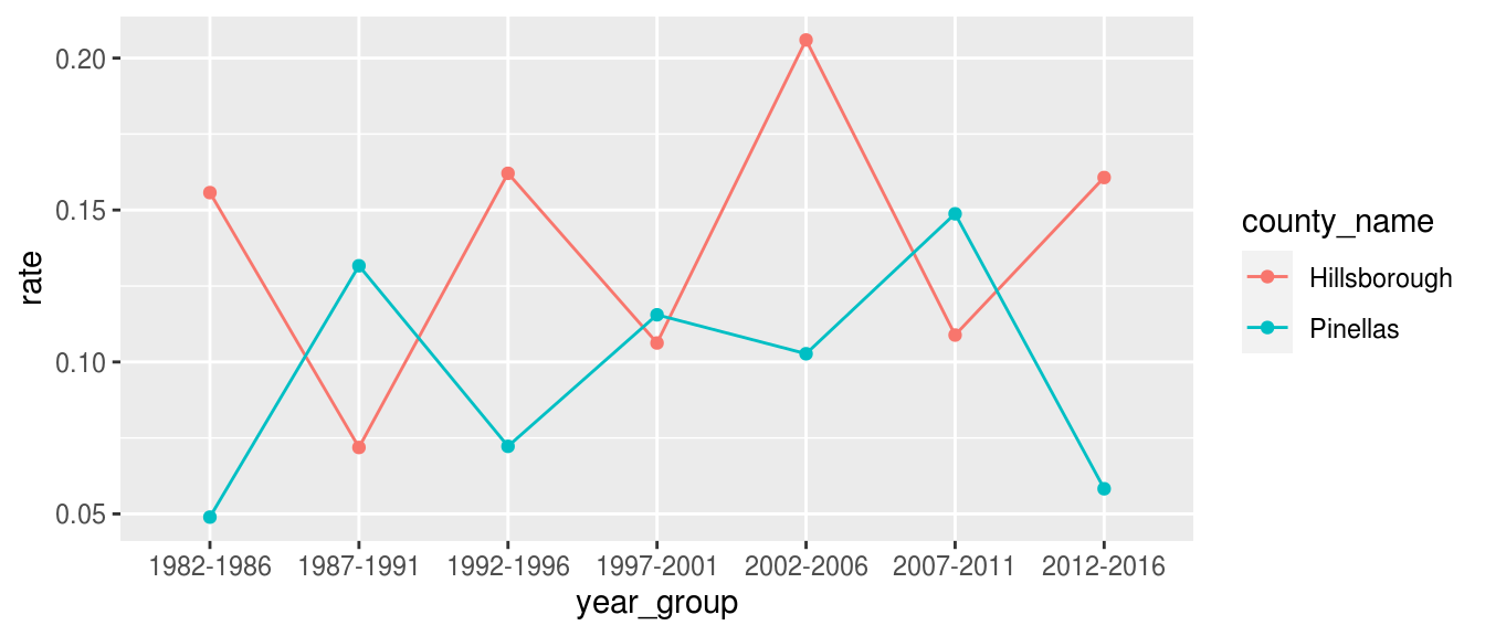
fcds_prostate <-
  fcds %>%
  # Filter to Prostate Cancer in two Florida counties
  filter(
    cancer_site_group == "Prostate Gland",
    county_name %in% c("Hillsborough", "Pinellas"),
    sex == "Male"
  ) %>%
  # Count incidences of Prostate Cancer
  count_fcds(county_name, cancer_site_group) %>%
  # Fill in missing age groups w.r.t. specified columns
  complete_age_groups(
    county_name, cancer_site_group, tidyr::nesting(year_group, year)
  ) %>%
  # Calculate age-adjusted rate from incidence
  age_adjust() %>%
  # Compute average yearly age-adjusted rate over 5 year range
  mutate(rate = rate / 5)

fcds_prostate
#> # A tibble: 14 x 7
#> # Groups:   county_name, cancer_site_group, year_group, year [14]
#>    county_name  cancer_site_group year_group year      n population   rate
#>    <fct>        <fct>             <fct>      <chr> <dbl>      <dbl>  <dbl>
#>  1 Hillsborough Prostate Gland    1982-1986  1984      5     731913 0.156
#>  2 Hillsborough Prostate Gland    1987-1991  1989      3     827378 0.0719
#>  3 Hillsborough Prostate Gland    1992-1996  1994      7     890958 0.162
#>  4 Hillsborough Prostate Gland    1997-2001  1999      5     984930 0.106
#>  5 Hillsborough Prostate Gland    2002-2006  2004     11    1108225 0.206
#>  6 Hillsborough Prostate Gland    2007-2011  2009      7    1214050 0.109
#>  7 Hillsborough Prostate Gland    2012-2016  2014     12    1319511 0.161
#>  8 Pinellas     Prostate Gland    1982-1986  1984      4     793633 0.0490
#>  9 Pinellas     Prostate Gland    1987-1991  1989      7     840882 0.132
#> 10 Pinellas     Prostate Gland    1992-1996  1994      5     884441 0.0723
#> 11 Pinellas     Prostate Gland    1997-2001  1999      7     917379 0.116
#> 12 Pinellas     Prostate Gland    2002-2006  2004      5     928305 0.103
#> 13 Pinellas     Prostate Gland    2007-2011  2009      9     915330 0.149
#> 14 Pinellas     Prostate Gland    2012-2016  2014      3     937933 0.0583
This data can readily be passed to ggplot2 for visualization.
library(ggplot2)

ggplot(fcds_prostate) +
  aes(year_group, rate, color = county_name, group = county_name) +
  geom_line() +
  geom_point()